5 Ways To Vlookup With Two Conditions

In the world of data analysis, being able to manipulate and extract information from large datasets is crucial. One of the most powerful tools in the Excel arsenal is the VLOOKUP function, which allows users to search for a value in a table and return a corresponding value from another column. However, what happens when you need to search for a value based on two conditions? In this article, we'll explore five ways to VLOOKUP with two conditions, making your data analysis tasks more efficient and accurate.

Understanding VLOOKUP

Before diving into the world of multiple conditions, let's quickly review how VLOOKUP works. The VLOOKUP function takes four arguments: the value you want to search for, the range of cells to search, the column number that contains the value you want to return, and an optional argument that specifies whether you want an exact match or an approximate match. The basic syntax of VLOOKUP is VLOOKUP(lookup_value, table_array, col_index_num, [range_lookup]).

Method 1: Using Multiple Criteria with the INDEX-MATCH Function

While VLOOKUP can't directly handle multiple criteria, the INDEX-MATCH function combination can. This method involves using the MATCH function to find the relative position of the first criterion, and then using the second criterion to find the relative position within the first criterion's range.

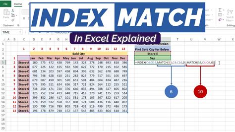
Here's an example formula: =INDEX(C:C, MATCH(1, (A:A="USA")*(B:B="NY"), 0)), where column A contains the country, column B contains the state, and column C contains the sales data.

Method 2: Using the FILTER Function (Excel 365 and Later)

The FILTER function, introduced in Excel 365, allows you to filter a range of data based on multiple criteria. You can use this function to filter your data and then use the VLOOKUP function to return the corresponding value.

Here's an example formula: =VLOOKUP("USA", FILTER(A:C, (A:A="USA")*(B:B="NY")), 3, FALSE), where column A contains the country, column B contains the state, and column C contains the sales data.

Method 3: Using Power Query

Power Query is a powerful data manipulation tool in Excel that allows you to create custom queries and load data into your workbook. You can use Power Query to filter your data based on multiple criteria and then load the results into your workbook.

Here's an example formula: = Table.SelectRows(#"Filtered Data", each [Country] = "USA" and [State] = "NY"), where #"Filtered Data" is the name of your query.

Method 4: Using the SUMIFS Function

While not directly related to VLOOKUP, the SUMIFS function can be used to sum values based on multiple criteria. This method involves using the SUMIFS function to sum the values in a specific column based on multiple criteria.

Here's an example formula: =SUMIFS(C:C, A:A, "USA", B:B, "NY"), where column A contains the country, column B contains the state, and column C contains the sales data.

Method 5: Using Multiple Criteria with the VLOOKUP Function (Helper Column)

This method involves creating a helper column that concatenates the two criteria and then using the VLOOKUP function to search for the concatenated value.

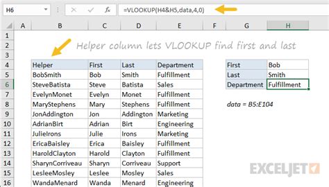
Here's an example formula: =VLOOKUP("USA-NY", A:C, 3, FALSE), where column A contains the country, column B contains the state, and column C contains the sales data. The helper column would contain the concatenated values, such as "USA-NY".

In conclusion, there are several ways to VLOOKUP with two conditions, each with its own advantages and disadvantages. By understanding these methods, you can choose the best approach for your specific data analysis task.

FAQs

What is the difference between VLOOKUP and INDEX-MATCH?

+

VLOOKUP searches for a value in a table and returns a corresponding value from another column, while INDEX-MATCH is a more flexible function that allows you to search for a value in a table and return a corresponding value from any column.

Can I use VLOOKUP with multiple criteria?

+

No, VLOOKUP can only search for a single value in a table. However, you can use the INDEX-MATCH function combination or the FILTER function to search for multiple criteria.

What is the best method for VLOOKUP with two conditions?

+

The best method depends on your specific data analysis task and the version of Excel you are using. If you are using Excel 365 or later, the FILTER function may be the most efficient method. Otherwise, the INDEX-MATCH function combination or the helper column method may be a better option.

We hope this article has been helpful in explaining the different methods for VLOOKUP with two conditions. Do you have any questions or comments about this topic? Please share them in the comments section below.